Improvement Research on RL Algorithms Based on Bayesian Dynamic Ensemble

Text Highlight Example

Abstract

In the field of deep reinforcement learning, algorithms are often constrained by challenges such as sample efficiency, model uncertainty, and dynamic changes in the environment. We introduces a novel reinforcement learning method utilizing Bayesian dynamic ensembles to address model uncertainty, thereby enhancing robustness and adaptability in varying environments. Our approach centers on a probabilistic network ensemble model that refines environmental dynamics and reward function estimations, incorporating a dynamic weight updating mechanism via Bayesian principles and importance sampling for improved model inference stability. Through extensive experiments, we demonstrate superior performance and generalizability of our method, particularly in bipedal locomotion tasks, and explore its robustness through ablation studies examining model resilience against extended imagining lengths and external noise.

Method

Model-Based Policy Optimization

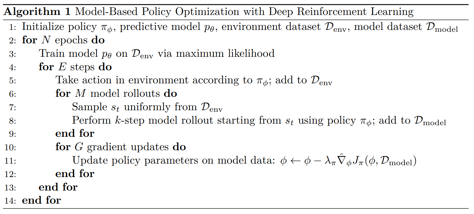
The Model-Based Policy Optimization (MBPO) algorithm proposes an innovative methodology for the effective utilization of environmental models. The principal concept underlying this approach is the implementation of short-horizon rollouts using the model, as opposed to conducting full trajectory simulations from the initial state. This strategy is encapsulated in the ‘branched rollout’ technique within MBPO. By generating new, short-term ‘branches’ on trajectories that have been previously sampled from the actual environment, the branched rollout method constrains the cumulative error inherent in the model, thus preserving the efficiency of the rollouts and enhancing the overall performance of the policy.

To effectively encapsulate model uncertainty, MBPO employs an ensemble methodology. More precisely, MBPO constructs an ensemble consisting of $ K $ neural networks, each with identical architecture. These networks receive state-action pairs as inputs and predict the mean vector and covariance matrix, characterizing the Gaussian distribution of the subsequent state. Each network within this ensemble is distinctively initialized and undergoes training on unique subsets of actual data. These subsets are sampled using the Bootstrap method throughout each iteration of training. This ensemble of probabilistic network models is represented as $ \hat{\mathcal{P}}_\theta = \{\hat{\mathcal{P}}_{\theta_1}, \hat{\mathcal{P}}_{\theta_2}, ..., \hat{\mathcal{P}}_{\theta_K}\} $. Here, each neural network is responsible for predicting the Gaussian distribution of the next state for a given state-action pair $ (s,a) $: $ \hat{\mathcal{P}}_{\theta_k}(s_{t+1} | s_t,a_t) = \mathcal{N}(\mu_{\theta_k} (s_t,a_t), \Sigma_{\theta_k} (s_t,a_t)) $. The training of these models utilizes a negative log-likelihood loss, defined as $ \mathcal{L}(\theta_{k}) = \sum_{t=1}^N [\mu_{\theta_k}(s_t,a_t)-s_{t+1}]^\top \Sigma_{\theta_k}^{-1}(s_t,a_t)[\mu_{\theta_k}(s_t,a_t)-s_{t+1}] + \log\det\Sigma_{\theta_k}(s_t,a_t) $. During the imagination phase, the ensemble of probabilistic dynamics models randomly selects a network, which then samples the subsequent state from the forecasted Gaussian distribution.

Bayesian Dynamic Ensemble

In MBPO, the stochasticity inherent in selecting a specific submodel from an ensemble during the imagination phase frequently results in diminished robustness across various tasks. This variability can undermine the reliability and performance consistency of the MBPO framework, particularly in complex environments where accurate prediction and decision-making are critical. To mitigate these challenges, we propose the implementation of a Bayesian dynamic ensemble approach, which takes inspiration from the Bayesian model averaging (BMA) technique.

So, during the imagination phase, we use a weighted average approach instead of randomly using the output of a submodel as the parameters of the Gaussian distribution, as done in the MBPO methods. Suppose we use the following notation to describe the reinforcement learning process:

$$ \begin{aligned} \mathbf x_{t} &= f(x_{t-1}) + \mathbf v_{t-1} \\ \mathbf y_{t} &= h_{\mathcal H_{t}}(x_t)+ \mathbf n_{t-1} \end{aligned} $$

where:

$$ \begin{aligned} \mathbf x_{t} &\triangleq \text{Concat} (s_{t}, a_{t})\\ \mathbf y_{t} &\triangleq \text{Concat} (s_{t+1}, r_{t}) \end{aligned} $$

$$ f \triangleq \text{the composite function of the transition function and policy function} $$ $$ h_{\mathcal H_{t}} \triangleq \text{a submodel of the ensemble model} $$

$$ \mathcal H_{t} \in \{ 1, 2, \ldots, M \} $$

If we want to calculate the weights for each model, it is crucial to derive the conditional probability $ \color{purple}{p(\mathcal H_{t-1} = m \mid y_{0:t-1})} $ from $ \color{green}{p(\mathcal H_{t} = m \mid y_{0:t})} $. This procedure enables continuous refinement of the model parameters at each timestep $ t $ and involves the following principal steps:

Exponential Smoothing with a Forgetting Factor: Begin by considering the transformation of the prior probability into a smoothed prior as dictated by the following equation, as detailed in 1: $$ \color{blue}{p(\mathcal H_{t} = m \mid y_{0:t-1})} \color{black}{=} \frac{\color{purple}{p(\mathcal H_{t-1} = m \mid y_{0:t-1})}^{\color{black}{\alpha}}}{\sum\limits_{j = 1}^{M} \color{purple}{p(\mathcal H_{t-1} = j \mid y_{0:t-1})}^{\color{black}{\alpha}}} $$ Here, $ \alpha $ represents a forgetting factor within the interval $ (0, 1) $ and serves as a hyperparameter to modulate the influence of historical data.
Application of Bayes’ Rule: Update the model’s belief about the current state by applying Bayes’ rule to incorporate new evidence: $$ \color{green}{p(\mathcal H_{t} = m \mid y_{0:t})} \color{black}{=} \frac{\color{blue}{p(\mathcal H_{t} = m \mid y_{0:t-1})} \color{red}{p_m(y_{t} \mid y_{0:t-1})}}{\sum\limits_{j=1}^{M} \color{blue}{p(\mathcal H_{t} = j \mid y_{0:t-1})} \color{red}{p_j(y_{t}\mid y_{0:t-1})}} $$
Computation of the Likelihood: The likelihood component $ \color{red}{p_m(y_{t} \mid y_{0:t-1})} $ is computed as follows, integrating over all possible states: $$ \color{red}{p_{m}(y_{t}\mid y_{0:t-1})} \color{black}= \int p_{m}(y_{t}\mid x_{t}) p(x_{t}\mid y_{0:t-1}) , dx_{t} $$ It can be estimated by importance sampling, as detailed in the subsequent section.

The above steps outline a structured approach to recursively updating the probabilistic beliefs about the system’s state by smoothly transitioning prior beliefs with new observational data, thus refining the model’s predictions over time.

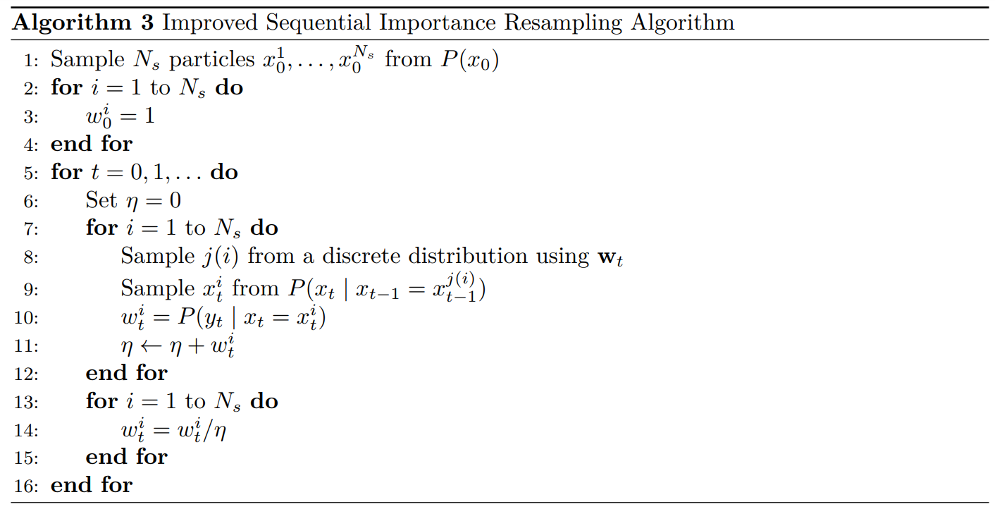
Sequential Importance Sampling

We can estimate it using sequential importance sampling as follows: $$ \color{red}{p_{m}(y_{t}\mid y_{0:t-1})} \color{black} \approx \sum\limits_{i=1}^{N_{s}} w_{t-1}^{i}p_{m}(y_{t} \mid x_{t}^{i}) $$

Experiments

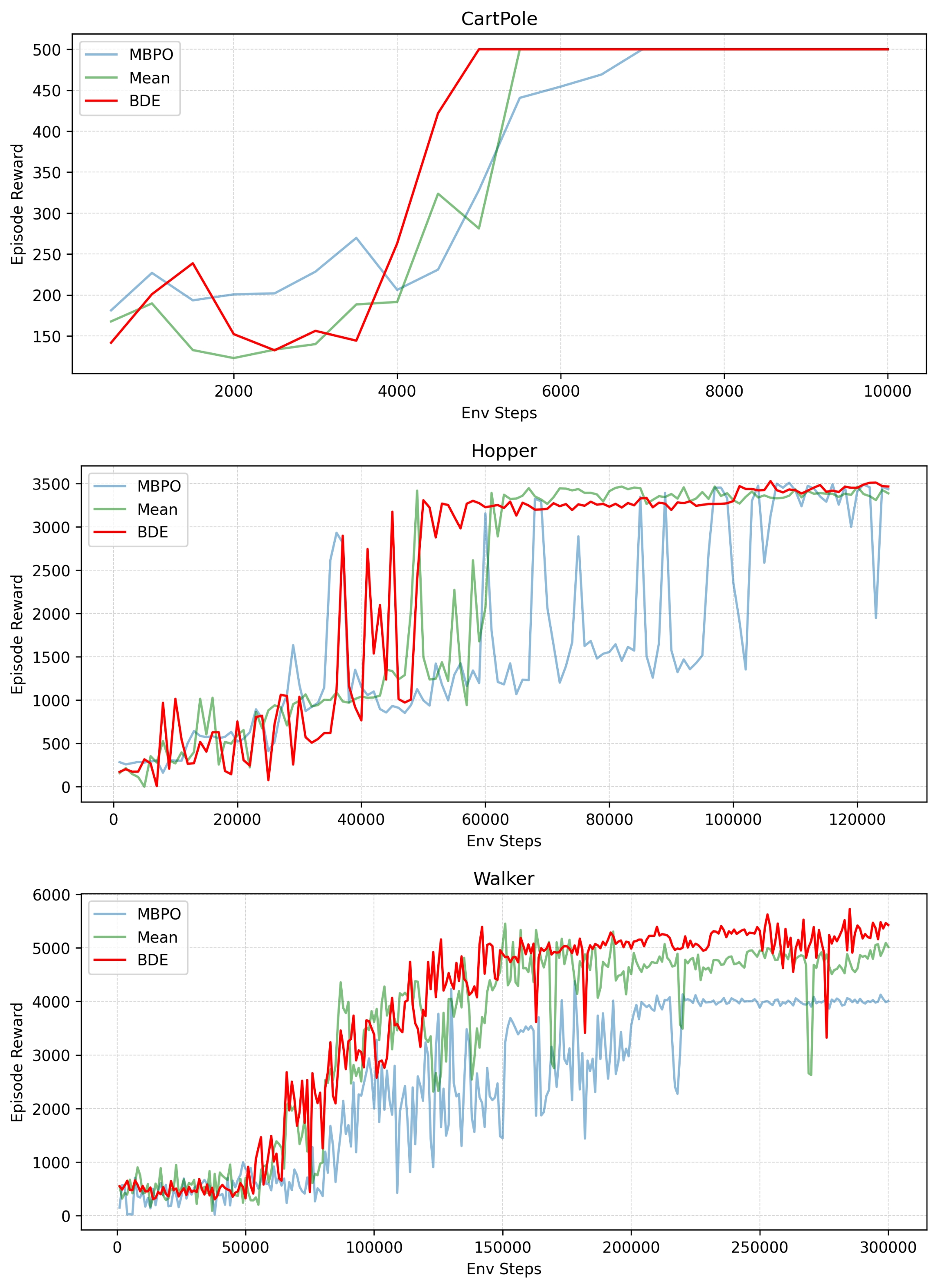
We have validated the effectiveness of our algorithm in classical control environment and the Mujoco environment. During the imagination phase, we employed different inference methods, namely MBPO and Simple Averaging. Our findings indicate that our approach generally outperforms the comparative methods.

Ablaition Study

To be updated…