Enhancing Training Robustness through Influence Measurement

In the realm of machine learning, the quest for robust and accurate models is incessant. One fundamental aspect of achieving model robustness is determining which data points in the training set should be removed and which high-quality, potentially unlabeled data points outside the training set should be included. To accomplish this, a proper metric is required to evaluate the importance of each datum in improving model performance. This paper proposes using the influence measure as a metric to assess the impact of training data on the model’s performance on the test set. Additionally, we introduce a data selection method for improving the training set and a dynamic active learning algorithm based on the influence measure. We demonstrate the effectiveness of the proposed algorithms through comprehensive simulations and real-world datasets.

Our paper has been accepted to ICLR 2025! 🎉

You can check out our paper at this link

Method

Data Trimming

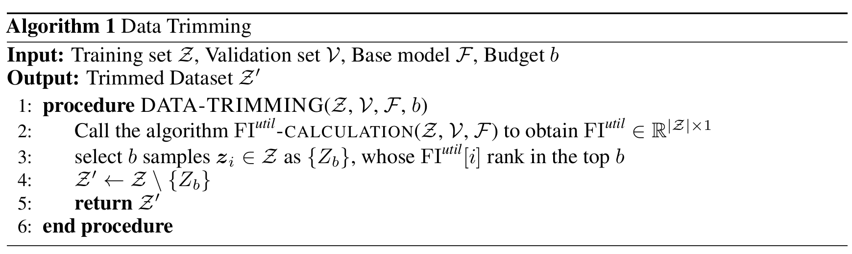
Given the training set \(\mathcal{Z}\), validation set \(\mathcal{V}\), base model \(\mathcal{F}\) and budget \(b\), the algorithm outputs the trimmed dataset \(\mathcal{Z}’\). The budget \(b\) specifies the number of samples to be deleted. The goal of this algorithm is to remove anomalous points from the training set based on \(\operatorname{FI}^{util}(\boldsymbol{z})\), thereby making the parameters learned by the model more stable and improving the model’s robustness on an unseen test set. In data trimming process, we first use Algorithm 3 to obtain the vector \(\operatorname{FI}^{\textit{util}}\), where the \(i\)-th element represents \(\operatorname{FI}^{\textit{util}}(\boldsymbol{z}_i)\), and \(\boldsymbol{z}_i\in\mathcal{Z}\). Next, we sort the \(n\) points in the training set in descending order of \(\operatorname{FI}^{\textit{util}}(\boldsymbol{z}_i)\). Finally, we remove the top \(b\) training samples with the highest \(\operatorname{FI}^{\textit{util}}(\boldsymbol{z}_i)\), and the remaining samples form the trimmed dataset \(\mathcal{Z}’\).

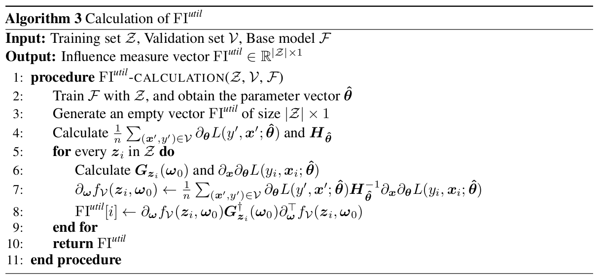
The above process can be summarized as the following algorithm.

Active Learning

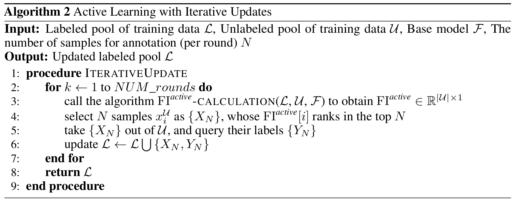
In the active learning application, we have a labeled pool of data \(\mathcal{L}\), an unlabeled pool of data \(\mathcal{U}\), along with a base model \(\mathcal{F}\). Our goal is to use \(\operatorname{FI}^{\textit{active}}(\boldsymbol{x}_{\textit{unlabel}})\) to select the most uncertain samples from \(\mathcal{U}\) to add to the training set and update the model in each round. \(N\) specifies the number of unlabelled samples to be included and the detailed algorithm in presented in Algorithm 2.

Experiments

Enhancing Training Robustness

Note: We will update the results with real-world data very soon. Meanwhile, you may refer to this link

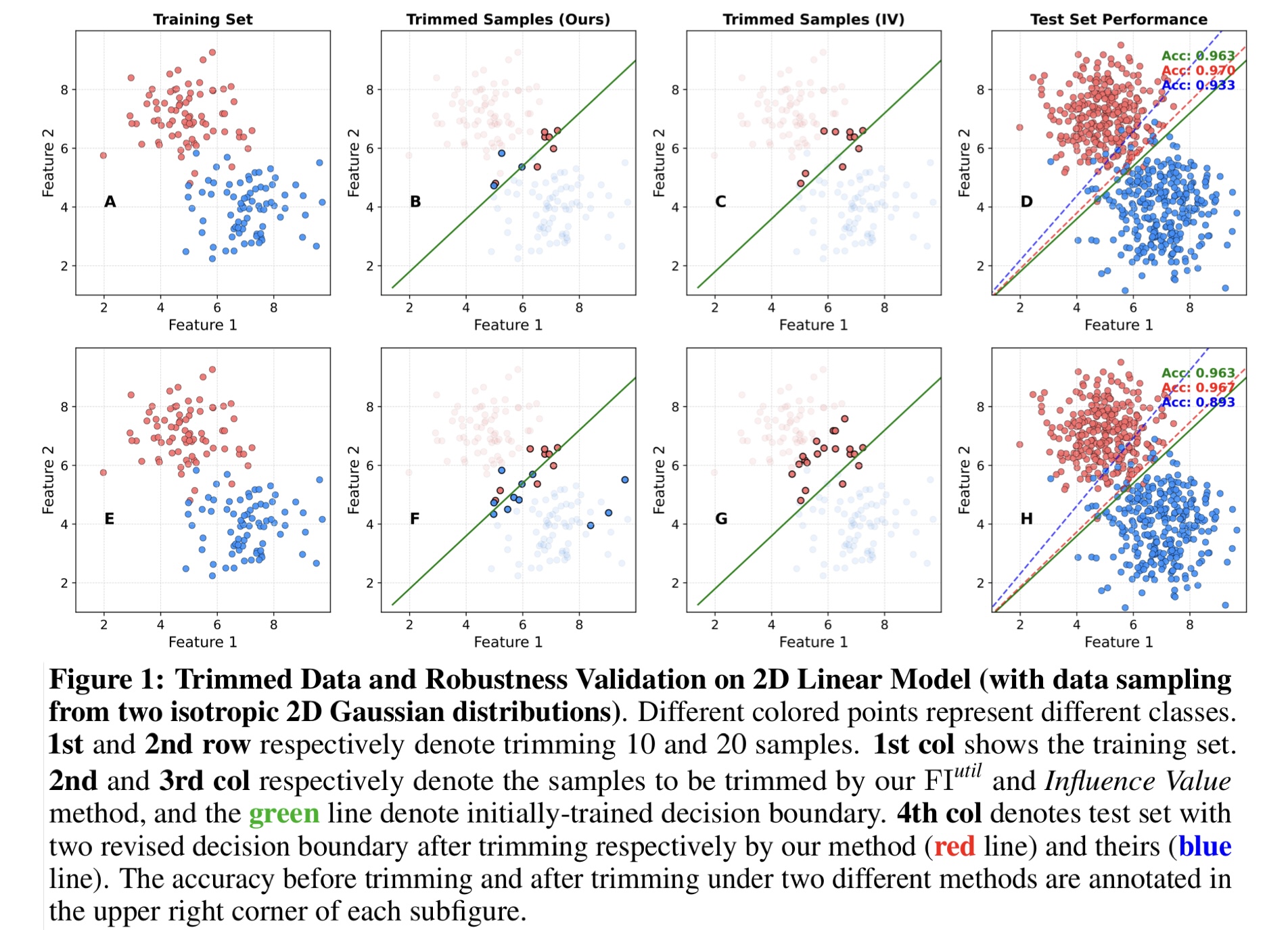
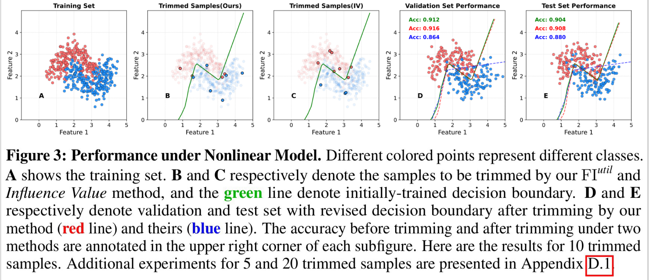
\(\text{FI}^{util}\) can effectively estimate each sample’s influence on model performance. We employ Algorithm 1 to trim “sensitive samples”. The latest method Influence Value, proposed by Chhabra et al.¹, serves as the primary baseline model for comparison in the experiments conducted in this subsection. We verify that our algorithm can better improve both linear and nonlinear models’ performance on synthetic datasets, even for some datasets with outliers.

Logistic regression is employed for this binary classification task. We first generate several datasets by sampling from two isotropic 2D Gaussian distributions. Each dataset consists of 150 training, 100 validation, and 600 test data. The experimental settings in this scenario are consistent with the study by Chhabra et al.¹. Our method improves model performance better than theirs in most cases by trimming 5, 10 and 20 samples respectively.Moreover, it can be observed that Influence Value tends to trim samples from a particular class under certain conditions, as shown in Figure 1 C and G.

Considering extending our method to nonlinear cases, we generate a non-linearly separable dataset via make_moons function from scikit-learn in Python, which consists of two interleaving half circles (often referred to as “moons”). We employ a neural network consisting of an input layer, two hidden layers with ReLU activation functions, and an output layer with a sigmoid activation function. As illustrated in Figure 3, it can be verified that our method can also improve training robustness of nonlinear model (similar to the previous analysis).

Active Learning

Note: The results need to be updated. We have conducted experiments on datasets such as UCI, CIFAR10, MNIST, EMNIST, and SVHN. Our method outperforms others like PowerBald ² and EPIG ³ under conditions of imbalanced and redundant data labels. We will update the results with real-world data very soon. Meanwhile, you may refer to this link

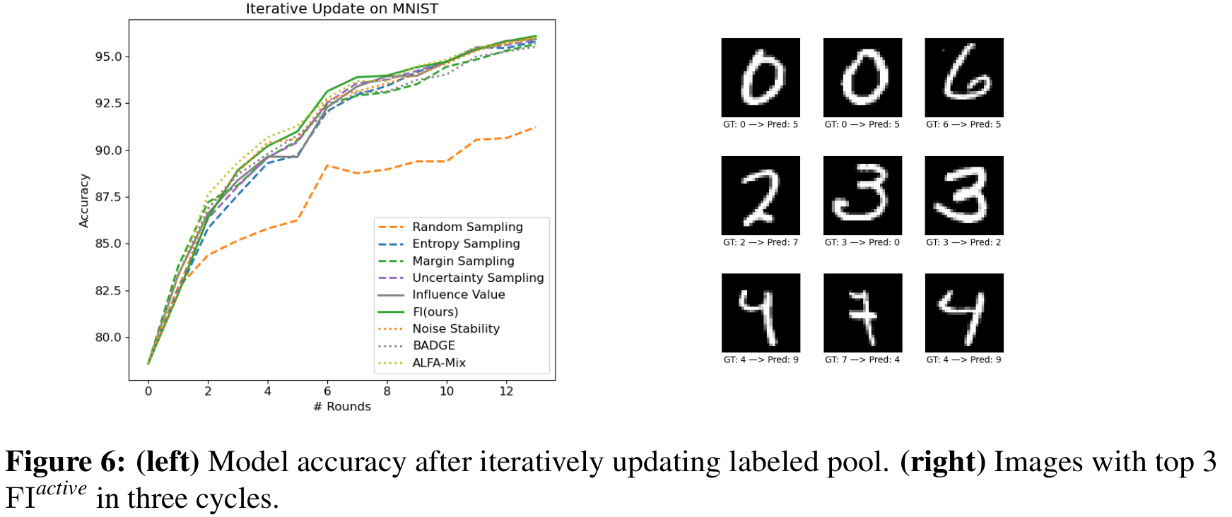
We have also conducted experiments on some real datasets and compared various methods of Active Learning. In image classification task, we implement a simple CNN on MNIST and validate the efficacy of our method. The simple CNN is designed with three convolutional layers(with batch normalization and ReLU activation), two fully connected layers, optional dropout regularization, and 10-class output. MNIST contains 60,000 training samples, and we only use a small subset for initially training model due to the simplicity of the task. The experiments are repeated for 5 circles, and 15 rounds of annotation queries is conducted for per circle. In each round, we select 20 samples with highest \(\operatorname{FI}^{\textit{active}}\) adding to the labeled pool. We present three rounds of annotation queries in Figure 6(left). It is evident that \(\operatorname{FI}^{\textit{active}}\) can identify those points that are difficult for the current model to “learn”. As is shown in Figure 6(right), our method maintains high accuracy throughout the most rounds and consistently ranks among the top-performing methods.